Please wait, while our marmots are preparing the hot chocolate…
 =WAT?=[image-full][top-left][darkened][*no-status][*black-bg]
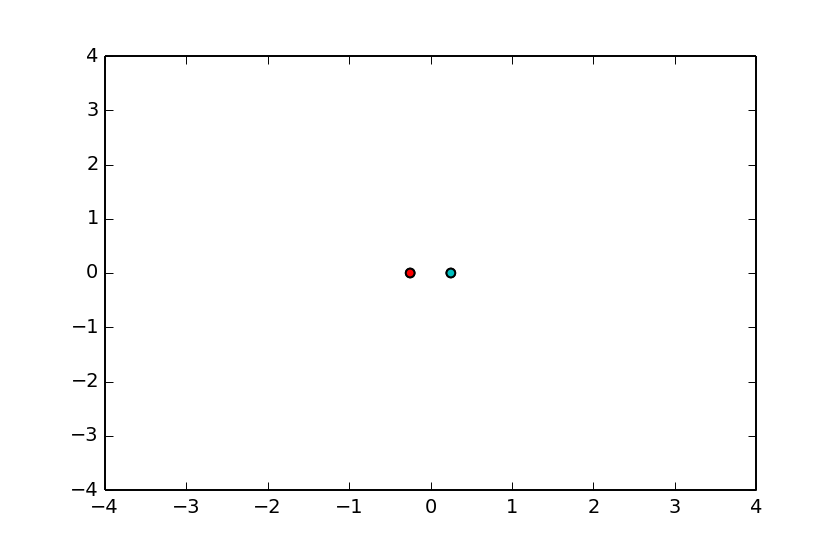
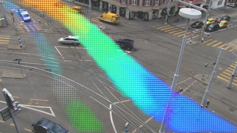
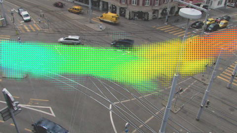
=Which pair of points are most similar?=
// color does not matter
@
=WAT?=[image-full][top-left][darkened][*no-status][*black-bg]
=Which pair of points are most similar?=
// color does not matter
@A: narrow 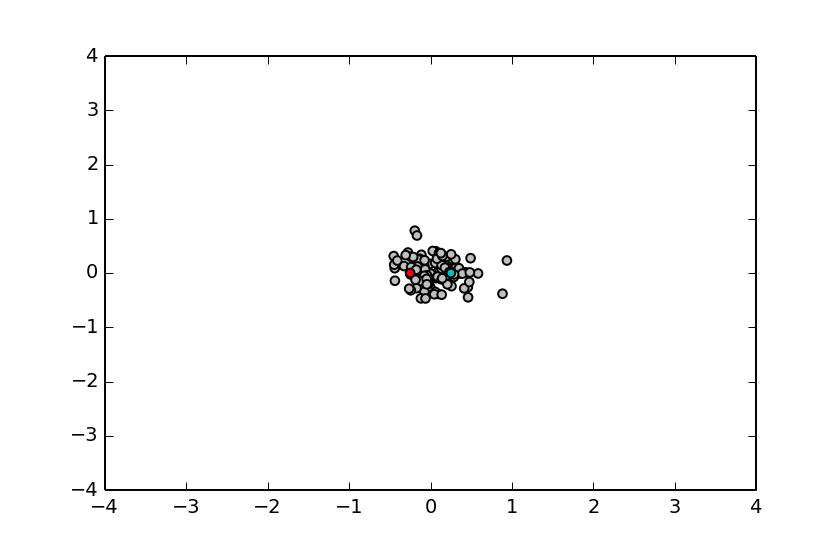
B: wide 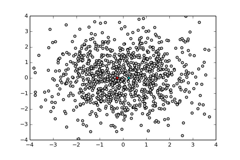
@context-aware comparison of points=[*no-status][image-full][bottom-left][darkened][*black-bg] // This is the intuition: comparing points given a global distribution (within a context) ==Probably Just Some Reminders== =Some Probability Rules, Measure Theory= @svg: floatrightbr,aa proba/potato-xandy.svg 245px 135px @svg: floatrightbr,bb proba/potato-xsumy.svg 245px 285px * Product rule[prod] ** $p(X, Y) = p(X|Y) \, p(Y)$ = $p(Y|X) \, p(X)$
* Marginalization, Sum rule[sum] ** $p(X) = \sum_{Y \in \mathcal{Y}} p(X,Y)$ ** $p(X) = \int_{Y \in \mathcal{Y}} p(X,Y)$ * Bayes rule[bayes] ** $p(Y|X) = \frac{p(X|Y) \, p(Y)}{p(X)}$ ** $p(X) = \sum_{Y\in \mathcal{Y}} p(X|Y) \, p(Y)$[denom] @anim-appear:800: .aa + .prod | .bb + .sum | .app | .bayes | .denom =Gaussian/Normal Distribution: basics= @svg: floatrightbr,fullabs gaussian/normal-distribution-stddev.svg 800px 500px =Gaussian/Normal Distribution: basics= @svg: floatrightbr gaussian/normal-distribution-stddev.svg 200px 200px * Normal Distribution or Gaussian Distribution[bb] ** $N(x|\mu,\sigma^2) = \frac{1}{\sqrt{2\pi \sigma^2}} exp(-\frac{(x-\mu)^2}{2 \sigma^2})$ ** Is-a probability density[bbb] ** $\int_{-\infty}^{+\infty} N(x|\mu,\sigma^2) dx = 1$[bbb] ** $N(x|\mu,\sigma^2) > 0$[bbb] * Parameters[cc] ** $\mu$: mean, $E[X] = \mu$ ** $\sigma^2$: variance, $E[(X -E[X])^2 ] = \sigma^2$ @anim-appear:800: .bb |.bbb |.cc =Multivariate Normal Distribution= * D-dimensional space: $x = \{x_1, ..., x_D\}$ * Probability distribution[slide] ** $N(x|\mu,\Sigma) = \frac{1}{\sqrt{(2\pi)^D \|\Sigma\|}}\; exp(-\frac{(x-\mu)^T\Sigma^{-1}(x-\mu)}{2})$ ** $\Sigma$: covariance matrix @svg: floatleft gaussian/multivariate-normal.svg 800px 250px @anim-appear:400: .hasSVG ==Probabilistic Models
and
Statistical Learning== =Maximum Likelihood Estimation= * We observe data points[slide] ** e.g., $\{ X_i \}_{i=1..N} \in R^N$ * We suppose a model (with parameters)[slide] ** e.g., $\forall i, X_i \sim N(.|\mu,\sigma^2)$ * We may try to maximize the likelihood
(find the “best parameters”)[slide] ** e.g., $\operatorname{arg max}_{\mu, \sigma^2} \mathcal{L}(\mu, \sigma^2 | X) = \operatorname{arg max}_{\mu, \sigma^2} p(X | \mu, \sigma^2) $ // what about priors? could be a two-hour discussion :) * We often maximize the log-likelihood[slide] ** e.g., $\operatorname{arg max}_{\mu, \sigma^2} \mathcal{L}(\mu, \sigma^2 | X) = \operatorname{arg max}_{\mu, \sigma^2} \log \mathcal{L}(\mu, \sigma^2 | X)$ ** e.g., $\log p(X | \mu, \sigma^2) = \log \prod_{i=1..N} p(X_i | \mu, \sigma^2) = \sum_{i=1..N} \log p(X_i | \mu, \sigma^2)$[slide] ** ⇒ equivalent, more convenient[slide] =Maximization of the Log-Likelihood= * We need to maximize $\log \mathcal{L}(\mu, \sigma^2 | X) = \log p(X | \mu, \sigma^2)$ * We set the derivatives to $0$ and solve it[slide] ** e.g., $\frac{\partial \log p(X | \mu, \sigma^2)}{\partial \mu} = 0$ and $\frac{\partial \log p(X | \mu, \sigma^2)}{\partial \sigma^2} = 0$ * Example, with a Gaussian: $p(X_i | \mu, \sigma^2) = \frac{1}{\sqrt{2\pi \sigma^2}} \exp^{(-\frac{(x-\mu)^2}{2 \sigma^2})}$[slide] ** we get $\mu = \frac{1}{N}\sum_{i=1..N} X_i$ and $\sigma^2 = \frac{1}{N}\sum_{i=1..N} (X_i - \mu)^2$ * The problem can also be written using the gradient[slide] ** $\nabla_{\mu,\sigma^2} \log \mathcal{L}(\mu, \sigma^2 | X) = \vec{0}$ ** the gradient is also called the Fisher Score, noted (here) $U_{X}$[slide] // $U_X(\mu, \sigma^2)$ =Understanding the Fisher Score= * Fisher Score: $\nabla_{\theta} \log \mathcal{L}(\theta | X) = U_X(\theta)$ * A function of $\theta$, considering $X$ fixed[slide] * How data points $X$ want to change the parameters $\theta$ ?[slide] // how the data wants to tune/update the model ** $X$ is known ** $\theta$ is known ** (considers a given model, with its parameters given) * (( Maximum likelihood estimation by gradient descent ))[slide] ** we look for the best model ($\theta$ unknown) ** evaluate the score (gradient) in the current estimate $\theta_t$ ** compute the next estimate $\theta_{t+1}$ =Fisher Kernel for Probabilistic Models= * Kernel trick ** goal: generalize linear algorithms to non-linear spaces ** given some input points ${X_i}$ (in any dimension)[slide][anim-continue] ** manipulate similarities given from a kernel $K(X_i, X_j)$
(instead of the points)[slide] * Fisher Kernel: a kernel from a prob. mod.[slide] ** compare data points ** in the context of a model with parameters $\theta$ (e.g., $\{\mu,\sigma^2\}$) ** $K(X_i, X_j) = U^T_{X_i} I^{-1} U_{X_j} = \nabla^T \log \mathcal{L}(\mu, \sigma^2 | X_i) \; I^{-1} \; \nabla \log \mathcal{L}(\mu, \sigma^2 | X_j)$[slide] // Actually I(\theta) ** $I$ : Fisher Information Matrix (normalizer)[slide] ** $I$ is a kind of normalization factor : $I = \E_{X}[U_{X} U_{X}^T]$[slide] ** “sometimes” $I_{ij} = -\E[\frac{\partial^2 \log \mathcal{L}(\theta)}{\partial \theta_i \partial \theta_j}]$[slide] =Which pair of points are most similar?= // color does not matter @
A: narrow
B: wide
@ =Example: mixture of gaussians=
 =Why $\frac{\partial \log \mathcal{L}}{\partial\theta}$ and not $\frac{\partial \log \mathcal{L}}{\partial X}$?=
@anim-appear:400: img
* Other: is $X$ continuous? map-able between instances? …[slide]
=Why $\frac{\partial \log \mathcal{L}}{\partial\theta}$ and not $\frac{\partial \mathcal{L}}{\partial \theta}$?=
* Derivative of the log: $\partial\log f = \frac{\partial f}{f}$[slide]
* ⇒ normalized/relative gradient[slide]
=Questions? Comments?=[image-fit][bottom-left][darkened][deck-status-fake-end]
@
=Why $\frac{\partial \log \mathcal{L}}{\partial\theta}$ and not $\frac{\partial \log \mathcal{L}}{\partial X}$?=
@anim-appear:400: img
* Other: is $X$ continuous? map-able between instances? …[slide]
=Why $\frac{\partial \log \mathcal{L}}{\partial\theta}$ and not $\frac{\partial \mathcal{L}}{\partial \theta}$?=
* Derivative of the log: $\partial\log f = \frac{\partial f}{f}$[slide]
* ⇒ normalized/relative gradient[slide]
=Questions? Comments?=[image-fit][bottom-left][darkened][deck-status-fake-end]
@
@
=Coffee Time!=[*no-status][image-full][top-left][darkened][*black-bg][deck-status-fake-end]
=Fisher Vectors for Image Classification ⇒=[title-slide][*no-status][image-full][*black-bg][top-left][darkened]
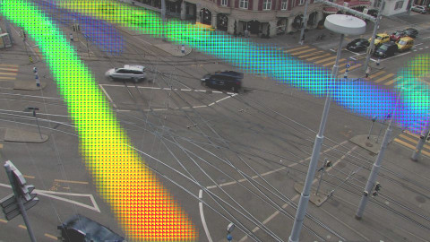
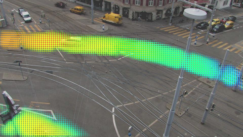
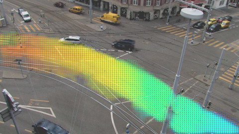
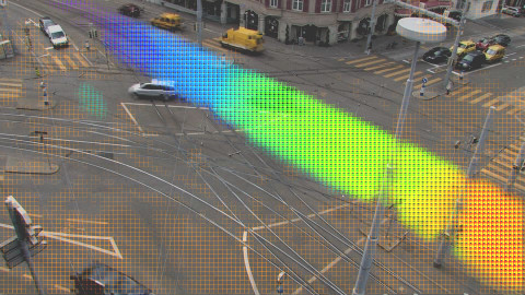
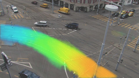
from Temporal Mixture Models=[*no-status][image-full][bottom-left][darkened][*black-bg] =Temporal Mixture Models=[*no-status][image-full][bottom-left][darkened][*black-bg] /* ============= TEMPORAL MIXTURE MODELS ============= */ =Task: Unsupervised Motif Mining= @SVG:owbg motif-mining/motif-mining-task.svg 750 400 @anim-appear:400: #layer1 + -#init | #layer2 | #layer3 | #layer7 | #layer4 | #layer6 | #layer5 /* ------------- PLSM THEN ---------------- */ =Probabilistic Latent Sequential Motifs= @svg:owbg past-temporal-approaches/plsm-process.svg 780px 500px @anim-appear:600: div.owbg | #g4915 | #rect3279 | #rect3279-0 | #rect3279-0-3 | #g5010 | -#rect3279,#rect3279-0,#rect3279-0-3,#g5010 | #g5123 | -#g5123 | -#g4915 | #g4915-8 | -#g4915-8 | #g4915-8-4 | -#g4915-8-4 =PLSM Graphical Model= @svg:owbg,floatright time-models/plsm-model-3.svg 300px 400px * Observations (time instant and word)
within a document: $(w,t_a)$ * Motifs: $\forall k \; \phi_k$ ≡ $p(w,t_r|z=k)$[slide] * Start/occurrences of motifs
within a document: $(z,t_s)$[slide] /* ------------- VIDEO CASE ---------------- */ =Video Case: Full Process= @SVG:owbg,space10 video-mining/process-full.svg 780px 470px @anim-appear:400: #layer1 | #shortll | #tdocetc @anim-appear:400: #shorttm | #layer7 | #layer5 @anim-appear:1000: #layer6 + -#layer3 + @#flow1 @anim-appear:600: @#flow2 | @#flow3 | -#layer6 + @#box1 + #layer2 @anim-appear:1000: @#box2 @anim-appear:1000: @#box3 /* ------------- VIDEO CASE: REPRESENTATION ---------------- */ =Video Case: motif representation= @SVG:fullsvg motif-repr/repr-motif.svg 780px 350px @anim-appear:400: #motiftable | #rt0 | #rt1 | #rt2 | #rt3 | #rt4 | #rt5 | #giffy | -#giffy | #arrow + #magic /* --------- KUETTEL --------- */ =Extracted Motifs: Kuettel3=[img3inwidth][shy]

 +
/* ------------- ACTION RECOGNITION IN VIDEOS ---------------- */
==Action Recognition in Videos==
=Motifs for Action Recognition=
@SVG:owbg action-recognition/explain.svg 780px 300px
// * Better generalization properties[title]
* Extract STIP
** spatiotemporal interest points
** like SIFT but with 2D+t cubes
* Learn temporal patterns of words (quantified STIP)
@CSS: .slide .hasSVG.dakth {margin-top: 15px;}
@CSS: .slide .hasSVG.kthpos {position: absolute; left:180px; top:58px;}
=Supervised Action Recognition=
@SVG:owbg action-recognition/overview-learning.svg 780 300
@SVG:owbg,dakth action-recognition/overview-test.svg 780 200
@SVG:wbg,kthpos action-recognition/kth_ntrain.svg 500 400
@anim-appear:700: .dakth | .kthpos
=Temporal Topic Models for Classification=
* Tested on action recognition
* To make it work for classification
** need to learn one model per class
** need to have very little learning data
/* -------- FISHER FOR PLSM --------- */
==Fisher Kernel/Vector
+
/* ------------- ACTION RECOGNITION IN VIDEOS ---------------- */
==Action Recognition in Videos==
=Motifs for Action Recognition=
@SVG:owbg action-recognition/explain.svg 780px 300px
// * Better generalization properties[title]
* Extract STIP
** spatiotemporal interest points
** like SIFT but with 2D+t cubes
* Learn temporal patterns of words (quantified STIP)
@CSS: .slide .hasSVG.dakth {margin-top: 15px;}
@CSS: .slide .hasSVG.kthpos {position: absolute; left:180px; top:58px;}
=Supervised Action Recognition=
@SVG:owbg action-recognition/overview-learning.svg 780 300
@SVG:owbg,dakth action-recognition/overview-test.svg 780 200
@SVG:wbg,kthpos action-recognition/kth_ntrain.svg 500 400
@anim-appear:700: .dakth | .kthpos
=Temporal Topic Models for Classification=
* Tested on action recognition
* To make it work for classification
** need to learn one model per class
** need to have very little learning data
/* -------- FISHER FOR PLSM --------- */
==Fisher Kernel/Vector From Temporal Topic Models== =Approach and Goal= * Goal[slide] ** improve discrimination power of temporal topic models (PLSM, ...) * Approach[slide] ** derive a Fisher Kernel from these models ** learn classifiers using the kernel ** and/or manipulate Fisher Vectors directly[slide] * Expected outcome[slide] ** no supervision at training ** better classification accuracy ** model-aware analysis of document similarity
(more in next slides) =Datasets for Classification of Time Series= * Pure classification ** action recognition *** STIP words across time ** music genre recognition *** spectrograms * Bird songs analysis, whales, … ** features *** spectrograms *** MFCC across time =Probabilistic Latent Sequential Motifs= // What are the parameters? @svg:owbg past-temporal-approaches/plsm-process.svg 780px 500px @anim-appear:300: div.owbg | #g4915 | #rect3279 | #rect3279-0 + #rect3279-0-3 + #g5010 + -#rect3279,#rect3279-0,#rect3279-0-3,#g5010 + #g5123 + -#g5123 + -#g4915 + #g4915-8 + -#g4915-8 + #g4915-8-4 + -#g4915-8-4 =Reminder: parameters in PLSM= @svg:owbg,floatright time-models/plsm-model-3.svg 300px 400px * Parameters[slide] ** global, motifs: $\forall k, \phi_k = p(w,t_r | k)$ ** per document: $\forall d, \theta_d = p(z,t_s | d)$ * Variation of motif weights ($\theta$) ** $p(z | d) = \sum_{t_s} p(z, t_s|d)$ ** Amount of motif in each document * Variation of motif shapes ($\phi$) ==The End==
/ − − will be replaced by the title
