Please wait, while the deck is loading…
{no} - {inlineblock center no custom1} -
-


a low-error classifier on
{no} - \begin{matrix} {R\_{\orange{P\_T}}(h)}&=&\mathbf{E}\_{(x^t,y^t)\sim \green{P\_S}}\frac{\orange{D\_T}(x^t)\orange{P\_T}(y^t|x^t)}{\green{D\_S}(x^t)\green{P\_S}(y^t|x^t)}\mathbf{I}\big[h(x^t)\ne y^t\big]\\\\ \\\\ &=&\mathbf{E}\_{(x^t,y^t)\sim \green{P\_S}}\frac{\orange{D\_T}(x^t)}{\green{D\_S}(x^t)}\mathbf{I}\big[h(x^t)\ne y^t\big]\\\\ \end{matrix} {latex no slide} - **⇒ Approach**: density estimation and instance re-weighting {no slide} // actually, it is simpler to estimate the density of the ratio - {notes notslide} - nice pres http://www.slideserve.com/Anita/sample-selection-bias ## Domain Adaptation − Domain Divergence {libyli} - {card dense libyli} - {inlineblock no} - Labeled
drawn *i.i.d.* from $\green{P_S}{}$ {c5} - {c1} - Unlabeled
drawn *i.i.d.* from $\orange{P_T}{}$ {c5} - $h$ is learned on the
 -
-  - Adaptation Bound [Ben-David et al., MLJ’10, NIPS’06] {card dense libyli}
- $\forall h\in\mathcal{H},\quad R\_{\orange{P\_T}}(h)\ \leq\ \; R\_{\green{P\_S}}(h)\ +\ \frac{1}{2} d\_{\mathcal{H}\;\Delta\;\mathcal{H}}(\green{D\_S},\orange{D\_T})\ +\ \nu $
- Domain divergence: $d\_{\mathcal{H}\;\Delta\;\mathcal{H}}(\green{D\_S},\orange{D\_T}) \;=\; 2 \sup\_{(h,h')\in\mathcal{H}^2} \Big| R\_{\orange{D\_T}}(h,h') - R\_{\green{D\_S}}(h,h')\Big| $
- Error of the joint optimal classifier: $\nu = \inf\_{h'\in\mathcal{H}}\big(R\_{\green{P\_S}}(h')+R\_{\orange{P\_T}}(h')\big)$
- {notes notslide}
- with some probability (1 - delta)
- H a symmetric hypothesis space
- More (by M. Sebban), epat slides
- about what is d_HH nips 07
# @copy:#plan: %+class:highlight: .dasa
## Unsupervised Visual Domain Adaptation Using Subspace Alignment − ICCV 2013
- Adaptation Bound [Ben-David et al., MLJ’10, NIPS’06] {card dense libyli}
- $\forall h\in\mathcal{H},\quad R\_{\orange{P\_T}}(h)\ \leq\ \; R\_{\green{P\_S}}(h)\ +\ \frac{1}{2} d\_{\mathcal{H}\;\Delta\;\mathcal{H}}(\green{D\_S},\orange{D\_T})\ +\ \nu $
- Domain divergence: $d\_{\mathcal{H}\;\Delta\;\mathcal{H}}(\green{D\_S},\orange{D\_T}) \;=\; 2 \sup\_{(h,h')\in\mathcal{H}^2} \Big| R\_{\orange{D\_T}}(h,h') - R\_{\green{D\_S}}(h,h')\Big| $
- Error of the joint optimal classifier: $\nu = \inf\_{h'\in\mathcal{H}}\big(R\_{\green{P\_S}}(h')+R\_{\orange{P\_T}}(h')\big)$
- {notes notslide}
- with some probability (1 - delta)
- H a symmetric hypothesis space
- More (by M. Sebban), epat slides
- about what is d_HH nips 07
# @copy:#plan: %+class:highlight: .dasa
## Unsupervised Visual Domain Adaptation Using Subspace Alignment − ICCV 2013 *Basura Fernando, Amaury Habrard, Marc Sebban, Tinne Tuytelaars (K.U. Leuven)* {paper libyli} - Intuition for unsupervised domain adaptation - principal components of the domains may be shared - principal components should be re-aligned - Principle - extract a
that aligns the
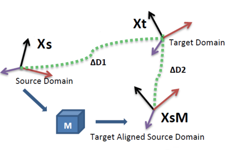 {no}
- {notes notslide}
- KULeuven
- More (by M. Sebban)
## Subspace Alignment − Algorithm
- Algorithm {card custom2 libyli}
- **Input:** Source data $\green{S}{}$, Target data $\orange{T}{}$, Source labels $\green{L\_S}{}$
- **Input:** Subspace dimension $d$ {no}
- **Output:** Predicted target labels $\orange{L\_T} {}$ {no}
- $\green{X\_S} \leftarrow PCA(\green{S},d)$ *(source subspace defined by the first d eigenvectors)*
- $\orange{X\_T} \leftarrow PCA(\orange{T},d)$ *(target subspace defined by the first d eigenvectors)*
- $M \leftarrow \green{X\_S}' \orange{X\_T}{}$ *(closed form alignment)*
- $X\_a \leftarrow \green{X\_S} M$ *(operator for aligning the source subspace to the target one)*
- $\gray{S\_a} = \green{S} X\_a$ *(new source data in the aligned space)*
- $\gray{T\_T} = \orange{T} \orange{X\_T}{}$ *(new target data in the aligned space)*
- $\orange{L\_T} \leftarrow Classifier(\gray{S\_a},\green{L\_S}, \gray{T\_T})$
- A natural similarity: $Sim(\mathbf{x}\_s,\mathbf{x}\_t)=\mathbf{x}\_sX\_SMX\_T' \mathbf{x}\_t'=\mathbf{x}\_sA \mathbf{x}\_t'$ {slide}
## Subspace Alignment − Experiments {libyli}
- *@svg:images-da-align/img-iccv13.svg 800px 200px* {no}
- Comparison on visual domain adaptation tasks // SURF, 800 words?
- adaptation from Office/Caltech-10 datasets (four domains to adapt)
- adaptation on ImageNet, LabelMe and Caltech-256 datasets: one is used as source and one as target
- Other methods
- Baseline 1: projection on the source subspace
- Baseline 2: projection on the target subspace
- 2 related methods:
- GFS [Gopalan et al.,ICCV'11] // Geodesic flow subspaces
- GFK [Gong et al., CVPR'12] // Geodesic flow kernel
## Subspace Alignment − Results {dense libyli}
- Office/Caltech-10 datasets {inlineblock}
- @svg:images-da-align/result1-NN-iccv13.svg 330px 250px
- @svg:images-da-align/result1-SVM-iccv13.svg 330px 250px
- ImageNet (I), LabelMe (L) and Caltech-256 (C) datasets {inlineblock}
- @svg:images-da-align/result2-NN-iccv13.svg 330px 130px
- @svg:images-da-align/result2-SVM-iccv13.svg 330px 130px
## Subspace Alignment − Recap. {#sarecap}
- Good
- Very simple and intuitive method
- Totally unsupervised
- Theoretical results for dimensionality detection
- Good results on computer vision datasets
- Can be combined with supervised information (future work)
- Bad {limitations}
- Cannot be directly kernelized to deal with non linearity
- Actually assumes that spaces are relatively close
- Ugly {limitations}
- Assumes that all the source and target examples are relevant
- **Idea:** *Select landmarks from both source and target domains to project the data in a common space using a kernel w.r.t those chosen landmarks. Then the subspace alignment is performed. {dense}* {hidden}
# @copy:#plan: %+class:highlight: .landmarks
# @copy:#sarecap: %+class:highlight: .limitations + %-class:hidden: .hidden
## Principle of Landmarks {libyli}
- JMLR 2013 − *Connecting the Dots with Landmarks:
{no}
- {notes notslide}
- KULeuven
- More (by M. Sebban)
## Subspace Alignment − Algorithm
- Algorithm {card custom2 libyli}
- **Input:** Source data $\green{S}{}$, Target data $\orange{T}{}$, Source labels $\green{L\_S}{}$
- **Input:** Subspace dimension $d$ {no}
- **Output:** Predicted target labels $\orange{L\_T} {}$ {no}
- $\green{X\_S} \leftarrow PCA(\green{S},d)$ *(source subspace defined by the first d eigenvectors)*
- $\orange{X\_T} \leftarrow PCA(\orange{T},d)$ *(target subspace defined by the first d eigenvectors)*
- $M \leftarrow \green{X\_S}' \orange{X\_T}{}$ *(closed form alignment)*
- $X\_a \leftarrow \green{X\_S} M$ *(operator for aligning the source subspace to the target one)*
- $\gray{S\_a} = \green{S} X\_a$ *(new source data in the aligned space)*
- $\gray{T\_T} = \orange{T} \orange{X\_T}{}$ *(new target data in the aligned space)*
- $\orange{L\_T} \leftarrow Classifier(\gray{S\_a},\green{L\_S}, \gray{T\_T})$
- A natural similarity: $Sim(\mathbf{x}\_s,\mathbf{x}\_t)=\mathbf{x}\_sX\_SMX\_T' \mathbf{x}\_t'=\mathbf{x}\_sA \mathbf{x}\_t'$ {slide}
## Subspace Alignment − Experiments {libyli}
- *@svg:images-da-align/img-iccv13.svg 800px 200px* {no}
- Comparison on visual domain adaptation tasks // SURF, 800 words?
- adaptation from Office/Caltech-10 datasets (four domains to adapt)
- adaptation on ImageNet, LabelMe and Caltech-256 datasets: one is used as source and one as target
- Other methods
- Baseline 1: projection on the source subspace
- Baseline 2: projection on the target subspace
- 2 related methods:
- GFS [Gopalan et al.,ICCV'11] // Geodesic flow subspaces
- GFK [Gong et al., CVPR'12] // Geodesic flow kernel
## Subspace Alignment − Results {dense libyli}
- Office/Caltech-10 datasets {inlineblock}
- @svg:images-da-align/result1-NN-iccv13.svg 330px 250px
- @svg:images-da-align/result1-SVM-iccv13.svg 330px 250px
- ImageNet (I), LabelMe (L) and Caltech-256 (C) datasets {inlineblock}
- @svg:images-da-align/result2-NN-iccv13.svg 330px 130px
- @svg:images-da-align/result2-SVM-iccv13.svg 330px 130px
## Subspace Alignment − Recap. {#sarecap}
- Good
- Very simple and intuitive method
- Totally unsupervised
- Theoretical results for dimensionality detection
- Good results on computer vision datasets
- Can be combined with supervised information (future work)
- Bad {limitations}
- Cannot be directly kernelized to deal with non linearity
- Actually assumes that spaces are relatively close
- Ugly {limitations}
- Assumes that all the source and target examples are relevant
- **Idea:** *Select landmarks from both source and target domains to project the data in a common space using a kernel w.r.t those chosen landmarks. Then the subspace alignment is performed. {dense}* {hidden}
# @copy:#plan: %+class:highlight: .landmarks
# @copy:#sarecap: %+class:highlight: .limitations + %-class:hidden: .hidden
## Principle of Landmarks {libyli}
- JMLR 2013 − *Connecting the Dots with Landmarks: Discriminatively Learning Domain-Invariant Features for Unsupervised Domain Adaptation{denser}* {no} - Boqing Gong, Kristen Grauman, Fei Sha - Principle: find source points (the landmarks) such that
the domains are similarly distributed “around” {inlineblock} - @svg:images-da-landmarks/landmarks1.svg 280px 100px - @svg:images-da-landmarks/landmarks2.svg 280px 100px - Optimization problem: $\min\_\alpha \left\\| \frac{1}{\sum\_m \alpha\_m } \sum\_m \alpha\_m \phi (x\_m) - \frac{1}{N} \sum\_n \phi(x\_n) \right\\|^2$ {dense} - {no} - $\alpha$: binary landmark indicator variables - $\phi(.)$: nonlinear mapping, maps every $x$ to a RKHS - minimize the difference in sample-means - \+ a constraint: *labels should be balanced among the landmarks* ## Landmarks-based Kernelized Subspace Alignment for Unsupervised DA − CVPR 2015
*Rahaf Aljundi, Rémi Emonet, Marc Sebban* {paper libyli} - Intuition for landmarks-based alignment - subspace alignment does not handle non-linearity - subspace alignment cannot “ignore” points - landmarks can be a useful to handle locality and non-linearity - Challenges - selecting landmarks in a unsupervised way - choosing the proper Gaussian-kernel scale @svg:images-da-landmarks/landmarks2.svg 700px 200px ## Proposed Approach − Workflow @svg:images-da-landmarks/workflow.svg 700px 400px - @anim: %viewbox:#zlandpro | %viewbox:#zpca | %viewbox:#zalign | %viewbox:#zclassify | %viewbox:#zall - Overall approach - 2 new steps: *landmark selection*, *projection* on landmarks - subspace alignment ## Multiscale Landmark Selection {libyli} - Select landmarks among all points, $\green{S} \cup \orange{T} {}$ - Greedy selection - consider each candidate point $c$ and a set of possible scales $s$ - criteria to promote the candidate - after projection on the candidate - the overlap between source and target distributions is above a threshold - Projection: a point is projected with $K(c, p)= \exp \left( \frac{-\left\|c - p\right\|^2}{2 s^2} \right)$ {dense} - Overlap {libyli} - project
 ## Contextually Constrained Deep Networks for Scene Labeling − BMVC 2015
 *Taygun Kekec, Rémi Emonet, Elisa Fromont, Alain Trémeau, Christian Wolf* {paper libyli} - Observation - state of the art uses deep CNN (conv. net.) - learning is patch-based, using the center label - training images are densely labeled - Idea - use labels in the patch to guide the network - force a part of the network to use the context (like an MRF) - @anim: .hasSVG @svg:cnn-context/cnn-app1.svg 800px 200px ## The Network // inspired by Farabet's paper @svg:cnn-context/cnns.svg 800px 400px ## Multi-Step Learning {libyli} @svg:cnn-context/cnn-app1.svg 800px 200px - Learn the context net (yellow) - Learn the dependent net (blue) - freeze the context net - use prediction, mixed with some ground truth (probability $\tau$) // small - Fine tuning - unfreeze the context net - no intermediate supervision - allow for co-adaptation ## Contextually Constrained − Results @svg:cnn-context/bmvc2014-results.svg 800px 400px ## Semantic Scene Parsing Using Inconsistent Labelings − CVPR 2016?
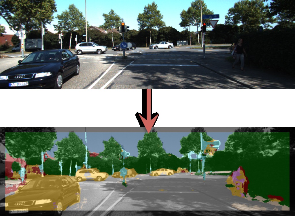
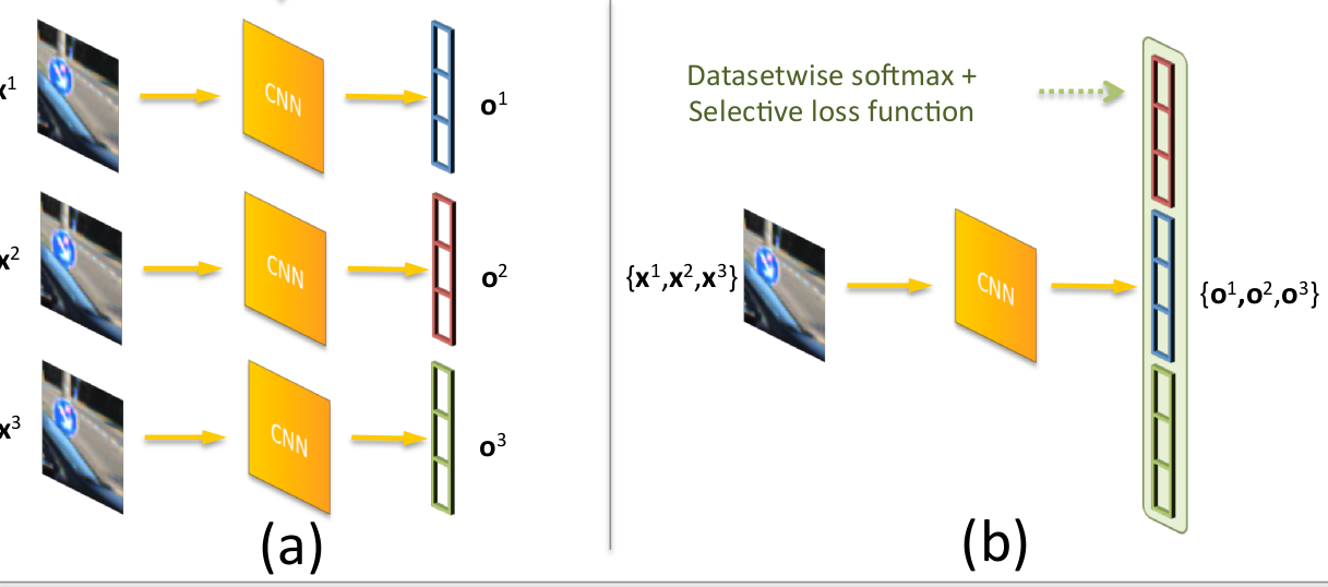
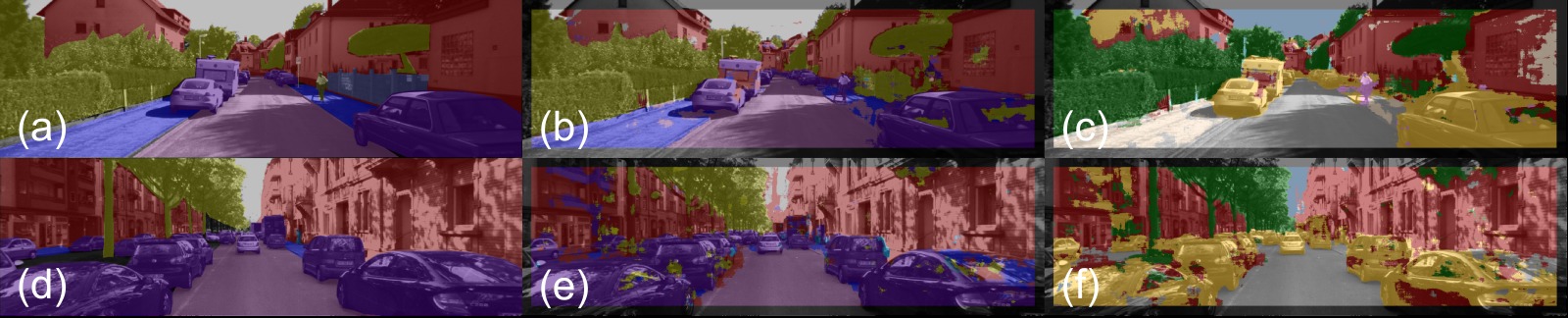
*Damien Fourure, et al.* {paper libyli} - Context: KITTI dataset - urban scenes recorded from a car - many sensors (RGB, stereo, laser, ...), different tasks - Observation (scene labeling on KITTI) {obs} - different groups labeled frames - they used different frames (mostly) and different labels - the quality/precision of annotations varies - @anim: .obs, .hasSVG - Goal - leverage all these annotations - improve segmentation on individual labelsets/datasets @svg:cnn-context/kitti-amount-labeled.svg 800px 200px ## Labels - 7 different label sets @svg:cnn-context/kitti-labels.svg 800px 200px @svg:cnn-context/kitti-amount-labeled.svg 800px 200px ## First Approach - a) Baseline: separate training - b) Joint Training - with datasetwise soft-max - with selective loss function
 ## Labels Correlation After Joint Training
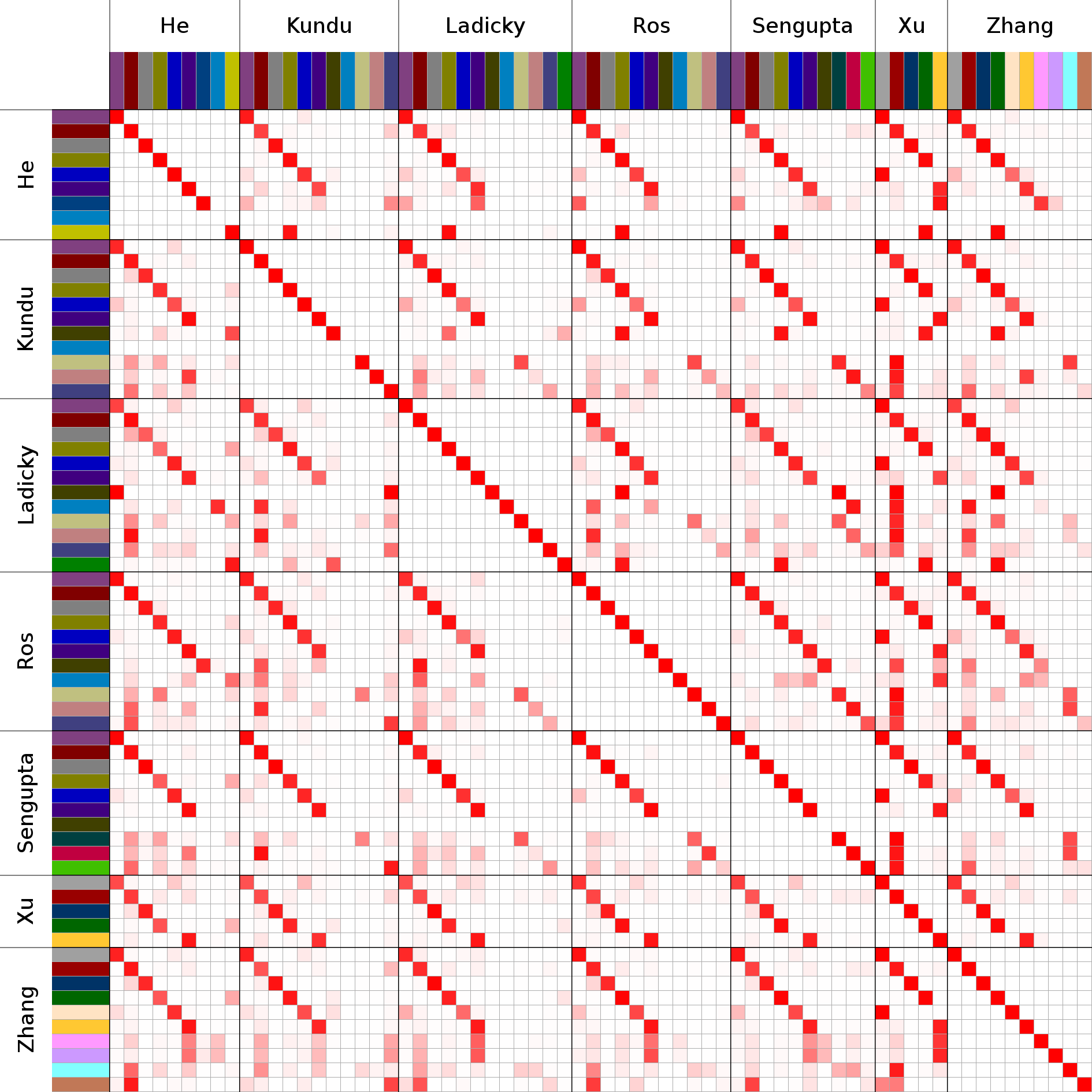 - Observing outputs
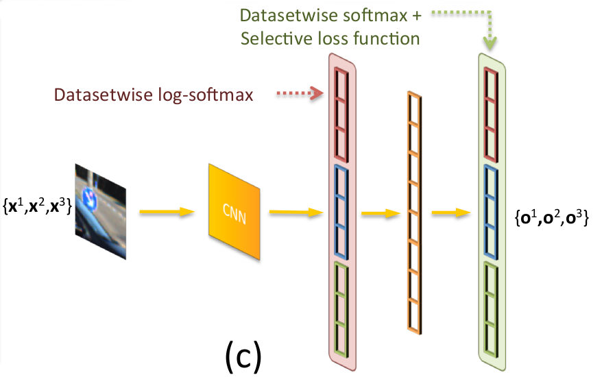
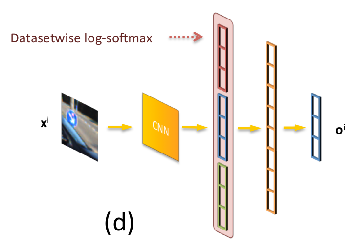
 after joint training {c5 libyli} - correlation across datasets - @anim: img - clear correspondence for some labels - one-to-many correspondences ## Exploiting Correlations after Joint Training - c) Joint Training with shared context {appc} - a single network to learn all correlations - d) Joint Training with individual context {appd} - a specialized network per labeling - @anim: .appc | .appd
 ## Joint Training − Results
@svg:cnn-context/kitti-results.svg 800px 300px
## Joint Training − Results
@svg:cnn-context/kitti-results.svg 800px 300px
 # @copy:#plan
# Thanks! More Questions?
# @copy:#plan
# Thanks! More Questions? **
{*no-status title-slide logos deck-status-fake-end} - - − # {deck-status-fake-end no-print} ## Supplementary slides − Links {no-print} - More details on DA (by M. Sebban) - Probabilistic Motif Mining - HCERES summary - VLTAMM, Multicam, etc - Bobbing 101
/ − − automatically replaced by the title
