Please wait while the marmots are preparing the hot chocolate…
- Marginalization, Sum rule{sum} - $p(X) = \sum_{Y \in \mathcal{Y}} p(X,Y)$ - $p(X) = \int_{Y \in \mathcal{Y}} p(X,Y)$ - Bayes rule{bayes} - $p(Y|X) = \frac{p(X|Y) \, p(Y)}{p(X)}$ - $p(X) = \sum_{Y\in \mathcal{Y}} p(X|Y) \, p(Y)${denom} - @anim: .aa + .prod | .bb + .sum | .app | .bayes | .denom # Gaussian/Normal Distribution ## Gaussian/Normal Distribution (1D) @svg: gaussian/normal-distribution-stddev.svg 800px 500px {floatrightbr fullabs} ## Gaussian/Normal Distribution (1D) @svg: gaussian/normal-distribution-stddev.svg 200px 200px {floatrightbr} - Normal Distribution or Gaussian Distribution{bb} - $\mathcal{N}(x|\mu,\sigma^2) = \frac{1}{\sqrt{2\pi \sigma^2}} exp(-\frac{(x-\mu)^2}{2 \sigma^2})$ - Is-a probability density{bbb} - $\int_{-\infty}^{+\infty} \mathcal{N}(x|\mu,\sigma^2) dx = 1${bbb} - $\mathcal{N}(x|\mu,\sigma^2) > 0${bbb} - Parameters{cc} - $\mu$: mean, $E[X] = \mu$ - $\sigma^2$: variance, $E[(X -E[X])^2 ] = \sigma^2$ - @anim: .bb |.bbb |.cc ## Multivariate Normal Distribution - D-dimensional space: $x = \{x\_1, ..., x_D\}$ - Probability distribution{slide} - $\mathcal{N}(x|\mu,\Sigma) = \frac{1}{\sqrt{(2\pi)^D \|\Sigma\|}}\; exp(-\frac{(x-\mu)^T\Sigma^{-1}(x-\mu)}{2})$ - $\Sigma$: covariance matrix - @anim: .hasSVG @svg: floatleft gaussian/multivariate-normal.svg 800px 250px # Gaussian Mixture Models ## Gaussian Mixture Model (1D) - Density: $p(x | \theta) = \sum_{k=1}^K w\_k \;\mathcal{N}(x|\mu\_k,\sigma\_k^2)$ {slide} - Parameters: $\theta = (w\_k, \mu\_k, {\sigma\_k}^2)_{k=1..K}$ {slide} @svg: gmm/two-gaussians-gmm.svg 800px 400px {unpadtop50} ## Sampling from a 2D GMM
 - {no}
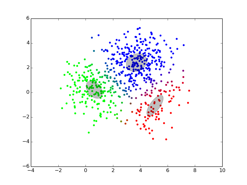
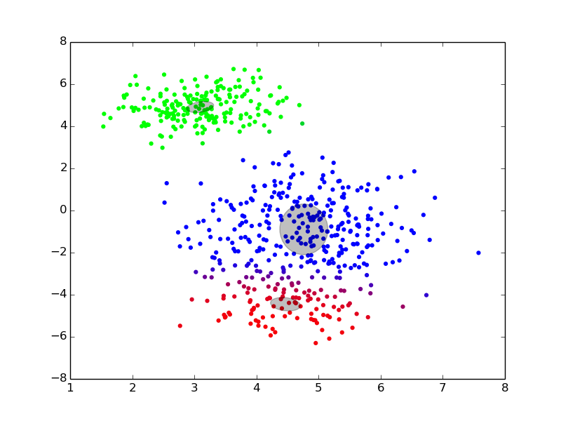
- Density: $p(x | \theta) = \sum_{k=1}^K w\_k \;\mathcal{N}(x|\mu\_k,\Sigma\_k)$
- Parameters: $\theta = (w\_k, \mu\_k, \Sigma\_k)_{k=1..K}$
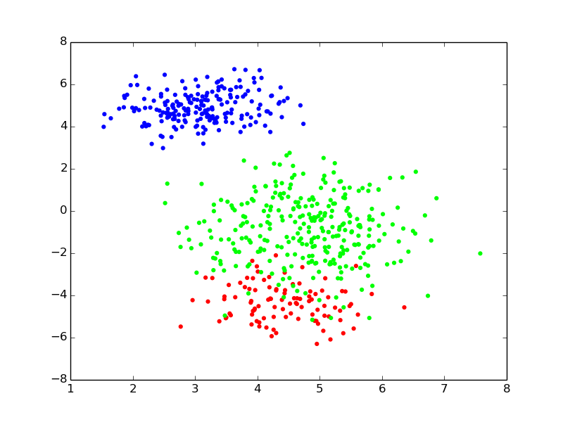
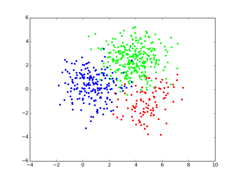
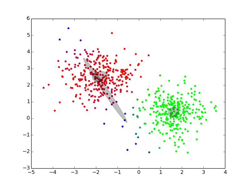
- For each point $i$ to be generated {clearboth}
- draw a **component index** (i.e., a color): $z_i \sim \operatorname{Categorical}(w)$
- draw its **position** from the component: $x\_i \sim \mathcal{N}(x|\mu\_{z\_i},\Sigma\_{z_i})$
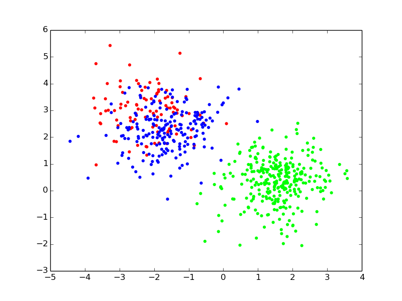
## Only Positions are Observed {pfree}
- {no}
- Density: $p(x | \theta) = \sum_{k=1}^K w\_k \;\mathcal{N}(x|\mu\_k,\Sigma\_k)$
- Parameters: $\theta = (w\_k, \mu\_k, \Sigma\_k)_{k=1..K}$
- For each point $i$ to be generated {clearboth}
- draw a **component index** (i.e., a color): $z_i \sim \operatorname{Categorical}(w)$
- draw its **position** from the component: $x\_i \sim \mathcal{N}(x|\mu\_{z\_i},\Sigma\_{z_i})$
## Only Positions are Observed {pfree}
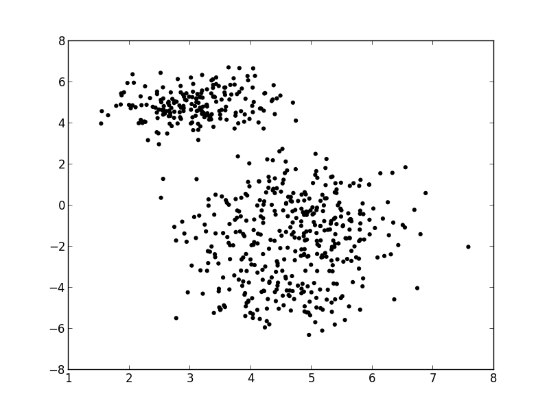 - For each point $i$ {clearboth}
- draw a component/color: $z_i \sim \operatorname{Categorical}(w)$
- draw a position: $x\_i \sim \mathcal{N}(x|\mu\_{z\_i},\Sigma\_{z_i})$
- Finding $z$ seems impossible,
- For each point $i$ {clearboth}
- draw a component/color: $z_i \sim \operatorname{Categorical}(w)$
- draw a position: $x\_i \sim \mathcal{N}(x|\mu\_{z\_i},\Sigma\_{z_i})$
- Finding $z$ seems impossible, finding the “best” $\theta$ might be feasible? {slide} ## GMM: Probabilistic Graphical Model @svg: graphical-models-dpgmm/dp-finite-no-prior.svg 800px 200px - Renamed - $w$ → $\beta$ (vector of component weights) - $(\mu\_k, \Sigma\_k)$ → $\phi_k$ (parameters of component $k$) - Reminder: for each point $i$ {clearboth} - draw a component/color: $z_i \sim \operatorname{Categorical}(\beta)$ - draw a position: $x\_i \sim \mathcal{N}(x|\phi\_{z\_i})$ # Learning/Inference
finding the best $\theta$ ## Maximum Likehood in GMM - From a set of observed points $x = \\{x\_i\\}\_{i=1..N}$ - Maximize the likelihood of the model {libyli} - NB: $\mathcal{L}(\theta | x) = p(x | \theta)$ - NB: $\operatorname{arg max}\_{\theta}\mathcal{L}(\theta | x) = \operatorname{arg max}\_{\theta}\log \mathcal{L}(\theta | x)$ - indep: $\log p(x | \theta) = \log \prod\_{i=1}^N p(x\_i | \theta) = \sum\_{i=1..N} \log p(x\_i | \theta)$ - mixture: $\log p(x | \theta) = \sum\_{i=1}^N \log \sum\_{k=1}^K w\_k \; \mathcal{N}(x\_i | \phi\_k)$ - No closed form expression → need to approximate{slide} # Expectation
Maximization ## Expectation-Maximization - Approximate inference by local optimization - converges to local optimum - needs a “good” initialization - Handling parameters and latent variables differently {slide} - single (point) estimate of the parameters $\theta$ - distribution estimate of the latent variables $z$ - Two-step iterative algorithm {libyli slide} - init: select a value for the parameters $\theta^0$ - E step: - compute the distribution over the latent variables - i.e., $\forall i,k \;\; p(z\_i = k | \theta^t)$ - these probabilities are called the “responsibilities” - M step: - find the best parameters $\theta$ given the responsibilities - i.e., $\theta^{t+1} = \operatorname{arg max}\_{\theta} $ ## EM iterations
 ## EM iterations
 ## EM iterations
 ## EM, Gibbs Sampling, Variational Inference {densetitle}
@svg: media/em-gibbs-variational.svg 800px 500px {unpademgibbsvariational}
- @anim: #header, #em | #eme | #emm | #gibbs | #gibbsloop | #cgibbs | #variational
# Beyond EM, using prior
## Prior on GMM
@svg: graphical-models-dpgmm/dp-finite-no-prior.svg 200px 200px {floatright light}
@svg: graphical-models-dpgmm/dp-finite.svg 200px 200px {floatright other}
- It's all about prior
- Intution in EM
- disappearing component
- “minimal” weight
- “minimal” variance
- {no notslide clearboth}
- We virtually add a few observations to each component {slide}
- $\alpha$: causes the weights $\beta$ to never be zero {slide}
- Dirichlet distribution: $\beta \sim \operatorname{Dirichlet}(\alpha)$
- $H$: adds some regularization on the variances $\Sigma_k$ {slide}
# … unfold
@svg: graphical-models-dpgmm/dp-finite.svg 200px 200px {other}
@svg: graphical-models-dpgmm/dp-finite-split.svg 200px 200px {other}
# Dirichlet Processes
## From GMM to DPGMM
@svg: graphical-models-dpgmm/dp-finite-split.svg 200px 200px {floatright light}
- Plain GMM
- the number of component $K$ needs to be know
- need to try multiple ones and do model selection
- (prior are not handled by EM)
- {no clearboth}
@svg: graphical-models-dpgmm/dp-split.svg 200px 200px {floatright other clearboth}
- Dirichlet Process GMM
- a GMM with an infinity of components
- with a proper prior
- cannot use EM for inference (infinite vectors)
# What is a Dirichlet Process, finally
## Dirichlet Process
@svg: graphical-models-dpgmm/dp-split.svg 200px 200px {floatright}
- What? {slide}
- a distribution over distributions
- a prior over distributions
- two parameters
- a scalar $\alpha$, the “concentration”
- a “base” distribution $H$ (any type)
- a draw from a DP is a countably infinite sum of Diracs
- Related formulations {libyli slide}
- Definition: complicated :)
- Stick breaking process (GEM)
- as shown on the graphical model
- e.g., a prior on the values of the weights
- Chinese Restaurant Process (CRP)
- how to generate the $z_i$, one by one, in sequence
- Polya Urn
##
## EM, Gibbs Sampling, Variational Inference {densetitle}
@svg: media/em-gibbs-variational.svg 800px 500px {unpademgibbsvariational}
- @anim: #header, #em | #eme | #emm | #gibbs | #gibbsloop | #cgibbs | #variational
# Beyond EM, using prior
## Prior on GMM
@svg: graphical-models-dpgmm/dp-finite-no-prior.svg 200px 200px {floatright light}
@svg: graphical-models-dpgmm/dp-finite.svg 200px 200px {floatright other}
- It's all about prior
- Intution in EM
- disappearing component
- “minimal” weight
- “minimal” variance
- {no notslide clearboth}
- We virtually add a few observations to each component {slide}
- $\alpha$: causes the weights $\beta$ to never be zero {slide}
- Dirichlet distribution: $\beta \sim \operatorname{Dirichlet}(\alpha)$
- $H$: adds some regularization on the variances $\Sigma_k$ {slide}
# … unfold
@svg: graphical-models-dpgmm/dp-finite.svg 200px 200px {other}
@svg: graphical-models-dpgmm/dp-finite-split.svg 200px 200px {other}
# Dirichlet Processes
## From GMM to DPGMM
@svg: graphical-models-dpgmm/dp-finite-split.svg 200px 200px {floatright light}
- Plain GMM
- the number of component $K$ needs to be know
- need to try multiple ones and do model selection
- (prior are not handled by EM)
- {no clearboth}
@svg: graphical-models-dpgmm/dp-split.svg 200px 200px {floatright other clearboth}
- Dirichlet Process GMM
- a GMM with an infinity of components
- with a proper prior
- cannot use EM for inference (infinite vectors)
# What is a Dirichlet Process, finally
## Dirichlet Process
@svg: graphical-models-dpgmm/dp-split.svg 200px 200px {floatright}
- What? {slide}
- a distribution over distributions
- a prior over distributions
- two parameters
- a scalar $\alpha$, the “concentration”
- a “base” distribution $H$ (any type)
- a draw from a DP is a countably infinite sum of Diracs
- Related formulations {libyli slide}
- Definition: complicated :)
- Stick breaking process (GEM)
- as shown on the graphical model
- e.g., a prior on the values of the weights
- Chinese Restaurant Process (CRP)
- how to generate the $z_i$, one by one, in sequence
- Polya Urn
## / − − will be replaced by the title
